Low IC, High Sharpe: The Quant Paradox Most Factor Models Get Wrong
Most quants chase high IC factors. That’s a mistake. This article breaks down, with real numbers, how low-IC quality signals can outperform through volatility suppression, regime behavior, and correct portfolio construction.
The Discovery That Changed Our Thinking
We recently ran a full-system backtest on our small-cap conviction scoring framework. At first glance, the results appeared internally inconsistent—almost contradictory.
Observed system-level metrics (Sep 2022 – Jan 2026):
| Metric | Value |
|---|---|
| Information Coefficient (IC) | +0.019 |
| Portfolio Sharpe Ratio | 0.72 |
| Hit Rate (positive months) | 70% |
| Maximum Drawdown | –7.2% |
An IC of +0.019 is, by conventional quant standards, weak. In most factor research, ICs below 0.05 are often dismissed as statistically insignificant. Interpreted naively, this suggests that the stock ranking mechanism is only marginally better than random at predicting relative outperformance.
Yet, the same system produced a Sharpe ratio of 0.72, with contained drawdowns of –7.2% and a 70% positive-period hit rate.
This raises an uncomfortable but important question:
How can a stock picker that appears “wrong” still produce a strong portfolio outcome?
The answer lies in a misunderstanding that is common even among experienced practitioners: Information Coefficient and Sharpe Ratio measure fundamentally different things. Optimizing one often degrades the other.
What Information Coefficient Actually Measures (and What It Doesn’t)
Information Coefficient (IC) is defined as the rank correlation between predicted scores and realized forward returns across a universe of stocks.
Formally, IC answers a single question:
“Do higher-scored stocks tend to outperform lower-scored stocks?”
A high IC (~0.10+) implies that relative ordering is preserved:
Score Rank → Return Rank1 → 1
2 → 3
3 → 2
A low IC (~0.02) implies that realized performance is largely scrambled:
Score Rank → Return Rank1 → 47
2 → 12
3 → 89
Critically, IC does not measure:
- Volatility of returns
- Correlation between selected stocks
- Tail risk or drawdown severity
- Return distribution skewness
- Compounding efficiency
IC is purely a ranking statistic. It evaluates relative prediction, not portfolio behavior.
What Sharpe Ratio Actually Measures
Sharpe Ratio is defined as:
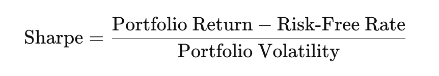
It answers a different question entirely:
“How much return is generated per unit of uncertainty?”
Sharpe can be improved through two independent levers:
- Increase returns (numerator)
- Reduce volatility (denominator)
This distinction is the key to resolving the apparent paradox.
Two Paths to Portfolio Performance
Path A: The Return Maximizer
Philosophy: Predict which stocks will outperform.
Typical factors:
- 52-week price momentum
- Earnings acceleration
- Revenue surprise
- Short-interest squeezes
Empirical characteristics:
- IC: 0.05 – 0.15
- Sharpe: 0.4 – 0.7
- Drawdowns: 30% – 50%
Momentum factors genuinely predict relative winners and are among the most robust signals in academic literature. However, they are volatile, regime-sensitive, and prone to sharp reversals.
Portfolio behavior:
- +40% up-years
- –25% down-years
- High emotional and capital stress
Path B: The Capital Preserver
Philosophy: Avoid stocks that will blow up.
Typical factors:
- Return on Equity (ROE)
- Return on Capital Employed (ROCE)
- Promoter / insider holding
- Dividend yield
- Low debt-to-equity
Empirical characteristics:
- IC: 0.01 – 0.04
- Sharpe: 0.6 – 1.0
- Drawdowns: 10% – 20%
Quality factors do not reliably identify winners. A stock with 25% ROE does not systematically outperform one with 15% ROE. Instead, these factors identify survivors.
Portfolio behavior:
- +15% up-years
- –8% down-years
- Psychologically and operationally sustainable
The Mathematics Behind the Paradox
Consider two hypothetical portfolios over four quarters.
Portfolio A: High IC, Momentum-Oriented
| Quarter | Return |
|---|---|
| Q1 | +25% |
| Q2 | –15% |
| Q3 | +30% |
| Q4 | –20% |
- Arithmetic mean: +5.0%
- Geometric mean: +3.2%
- Volatility: 24%
- Sharpe: 0.21
Portfolio B: Low IC, Quality-Oriented
| Quarter | Return |
|---|---|
| Q1 | +8% |
| Q2 | +2% |
| Q3 | +10% |
| Q4 | –3% |
- Arithmetic mean: +4.25%
- Geometric mean: +4.2%
- Volatility: 5.5%
- Sharpe: 0.77
Despite lower average returns, Portfolio B compounds more efficiently due to volatility suppression.
The quality factors did not pick winners. They filtered out bombs.
Regime Dependence: When Low IC Still Works
In our empirical backtest, IC varied materially across regimes:
| Regime | IC |
|---|---|
| NEUTRAL | +0.019 |
| RISK-ON | –0.057 |
During aggressive bull phases, low-quality, speculative stocks outperform. Quality filters actively select underperformers in such regimes.
Yet the system remained viable because:
- RISK-ON periods are episodic
- Downside protection during corrections dominates long-term compounding
- Loss asymmetry matters:
- –50% requires +100% to recover
- –20% requires only +25%
Avoiding catastrophic losses has higher long-term impact than capturing extreme upside.
Factor Design Is a Menu of Trade-offs
| Factor Type | IC to Returns | Volatility Reduction | Primary Objective |
|---|---|---|---|
| Momentum | +0.08 | Low | Return maximization |
| Value | +0.04 | Medium | Balanced |
| Quality | +0.02 | High | Capital preservation |
| Low Volatility | –0.02 | Very High | Risk minimization |
Notably, low-volatility factors often exhibit negative IC, yet frequently outperform on a risk-adjusted basis due to dominant volatility reduction.
Portfolio Construction Must Match IC
Factor choice is only half the equation. Portfolio construction determines whether the factor’s edge is amplified or destroyed.
High IC Factors (Momentum)
- 8–10 stocks
- ≤15% per position
- Score-weighted sizing
- HHI: 1000–1500
Concentration amplifies predictive signals.
Low IC Factors (Quality)
- 15–20 stocks
- ≤6% per position
- Equal-weighted sizing
- HHI: 400–700
Diversification amplifies risk filtering.
The Concentration Trap (Empirical Results)
| Portfolio Size | Minimum IC Needed for Concentration |
|---|---|
| 5 stocks | >0.08 |
| 8 stocks | >0.05 |
| 10 stocks | >0.04 |
| 15+ stocks | >0.02 |
With an observed IC of 0.019:
- 5-stock portfolio: Sharpe 0.34 (–53% vs optimal)
- 15-stock portfolio: Sharpe 0.72 (optimal)
Concentrating low-IC signals concentrates idiosyncratic risk, not alpha.
A Simple Decision Framework
Before designing any strategy, ask:
“When I am wrong about a stock, what happens?”
- Underperforms by 5–10%
→ High IC likely
→ Concentration justified - Potential permanent impairment
→ Low IC expected
→ Diversification essential
How Institutions Actually Use This
Professional allocators separate objectives:
| Sleeve | Objective | Factors | IC | Portfolio |
|---|---|---|---|---|
| Alpha | Maximize returns | Momentum, Growth | ~0.08 | Concentrated |
| Core | Benchmark-like | Value, Quality | ~0.03 | Diversified |
| Defense | Drawdown control | Low Vol, Dividend | ~0.01 | Very diversified |
They do not ask which factor is “best.”
They ask what role it plays.
Conclusion: The IC–Sharpe Trade-off Is a Feature, Not a Bug
Our small-cap system exhibits:
- IC: +0.019
- Sharpe: 0.72
- Max Drawdown: –7.2%
The correct interpretation is not “the scoring is broken.”
It is:
“The scoring is optimized for capital preservation, and it is behaving exactly as designed.”
Key takeaways:
- IC measures return prediction; Sharpe measures risk-adjusted outcomes.
- Quality factors have low IC by construction.
- Portfolio concentration must be justified by IC.
- Misaligned construction destroys value.
- Strategy design begins with objective clarity, not factor worship.
Sometimes the best portfolio comes from a stock picker that looks like a coin flip—as long as the coin never lands on catastrophe.
This analysis is based on empirical backtesting of a small-cap Indian equity strategy from September 2022 to January 2026. Past performance does not guarantee future results. Factor behavior is cyclical and regime-dependent.